JPL Spectroscopy Queries (astroquery.jplspec)
Getting Started
The JPLSpec module provides a query interface for JPL Molecular
Spectroscopy Catalog. The
module outputs the results that would arise from the browser form,
using similar search criteria as the ones found in the form, and presents
the output as a Table.
Examples
Querying the catalog
The default option to return the query payload is set to false, in the following examples we have explicitly set it to False and True to show the what each setting yields:
>>> from astroquery.jplspec import JPLSpec
>>> import astropy.units as u
>>> response = JPLSpec.query_lines(min_frequency=100 * u.GHz,
...                                max_frequency=1000 * u.GHz,
...                                min_strength=-500,
...                                molecule="28001 CO",
...                                get_query_payload=False)
>>> print(response)
    FREQ     ERR    LGINT   DR   ELO   GUP  TAG   QNFMT QN' QN"
    MHz      MHz   nm2 MHz      1 / cm
----------- ------ ------- --- -------- --- ------ ----- --- ---
115271.2018 0.0005 -5.0105   2      0.0   3 -28001   101   1   0
   230538.0 0.0005 -4.1197   2    3.845   5 -28001   101   2   1
345795.9899 0.0005 -3.6118   2   11.535   7 -28001   101   3   2
461040.7682 0.0005 -3.2657   2  23.0695   9 -28001   101   4   3
576267.9305 0.0005 -3.0118   2  38.4481  11 -28001   101   5   4
691473.0763 0.0005 -2.8193   2  57.6704  13 -28001   101   6   5
 806651.806  0.005 -2.6716   2  80.7354  15 -28001   101   7   6
   921799.7  0.005  -2.559   2 107.6424  17 -28001   101   8   7
The following example, with get_query_payload = True, returns the payload:
>>> response = JPLSpec.query_lines(min_frequency=100 * u.GHz,
...                                   max_frequency=1000 * u.GHz,
...                                   min_strength=-500,
...                                   molecule="28001 CO",
...                                   get_query_payload=True)
>>> print(response)
[('MinNu', 100.0), ('MaxNu', 1000.0), ('MaxLines', 2000), ('UnitNu', 'GHz'), ('StrLim', -500), ('Mol', '28001 CO')]
The units of the columns of the query can be displayed by calling
response.info:
>>> response = JPLSpec.query_lines(min_frequency=100 * u.GHz,
...                                max_frequency=1000 * u.GHz,
...                                min_strength=-500,
...                                molecule="28001 CO")
>>> print(response.info)
   <Table length=8>
  name  dtype    unit
 ----- ------- -------
  FREQ float64     MHz
   ERR float64     MHz
 LGINT float64 nm2 MHz
    DR   int64
   ELO float64  1 / cm
   GUP   int64
   TAG   int64
 QNFMT   int64
   QN'   int64
   QN"   int64
These come in handy for converting to other units easily, an example using a simplified version of the data above is shown below:
>>> print (response['FREQ', 'ERR', 'ELO'])
    FREQ     ERR     ELO
    MHz      MHz    1 / cm
----------- ------ --------
115271.2018 0.0005      0.0
   230538.0 0.0005    3.845
345795.9899 0.0005   11.535
461040.7682 0.0005  23.0695
576267.9305 0.0005  38.4481
691473.0763 0.0005  57.6704
 806651.806  0.005  80.7354
   921799.7  0.005 107.6424
>>> response['FREQ'].quantity
<Quantity [115271.2018, 230538.    , 345795.9899, 461040.7682, 576267.9305, 691473.0763, 806651.806 , 921799.7   ] MHz>
>>> response['FREQ'].to('GHz')
<Quantity [115.2712018, 230.538    , 345.7959899, 461.0407682, 576.2679305, 691.4730763, 806.651806 , 921.7997   ] GHz>
The parameters and response keys are described in detail under the Reference/API section.
Looking Up More Information from the catdir.cat file
If you have found a molecule you are interested in, the TAG field in the results provides enough information to access specific molecule information such as the partition functions at different temperatures. Keep in mind that a negative TAG value signifies that the line frequency has been measured in the laboratory
>>> import matplotlib.pyplot as plt
>>> from astroquery.jplspec import JPLSpec
>>> result = JPLSpec.get_species_table()
>>> mol = result[result['TAG'] == 28001] #do not include signs of TAG for this
>>> print(mol)
 TAG  NAME NLINE QLOG1  QLOG2  QLOG3 QLOG4  QLOG5  QLOG6  QLOG7  VER
----- ---- ----- ------ ------ ----- ------ ------ ------ ------ ---
28001   CO    91 2.0369 1.9123 1.737 1.4386 1.1429 0.8526 0.5733  4*
You can also access the temperature of the partition function through metadata:
>>> result['QLOG2'].meta
{'Temperature (K)': 225}
>>> result.meta
{'Temperature (K)': [300, 225, 150, 75, 37.5, 18.5,
                     9.375]}
One of the advantages of using JPLSpec is the availability in the catalog of the partition function at different temperatures for the molecules. As a continuation of the example above, an example that accesses and plots the partition function against the temperatures found in the metadata is shown below:
>>> temp = result.meta['Temperature (K)']
>>> part = list(mol['QLOG1','QLOG2','QLOG3', 'QLOG4', 'QLOG5','QLOG6',
...                 'QLOG7'][0])
>>> plt.scatter(temp,part)
>>> plt.xlabel('Temperature (K)')
>>> plt.ylabel('Partition Function Value')
>>> plt.title('Parititon Fn vs Temp')
>>> plt.show()
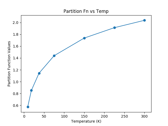
The resulting plot from the example above
For non-linear molecules like H2O, curve fitting methods can be used to
calculate production rates at different temperatures with the proportionality:
a*T**(3./2.). Calling the process above for the H2O molecule (instead of
for the CO molecule) we can continue to determine the partition function at
other temperatures using curve fitting models:
>>> from scipy.optimize import curve_fit
>>> def f(T,a):
        return np.log10(a*T**(1.5))
>>> param, cov = curve_fit(f,temp,part)
>>> print(param)
# array([0.03676998])
>>> x = np.linspace(5,305)
>>> y = f(x,0.03676998)
>>> plt.scatter(temp,part,c='r')
>>> plt.plot(x,y,'k')
>>> plt.title('Partition Function vs Temperature')
>>> plt.xlabel('Temperature')
>>> plt.ylabel('Log10 of Partition Function')
>>> plt.show()
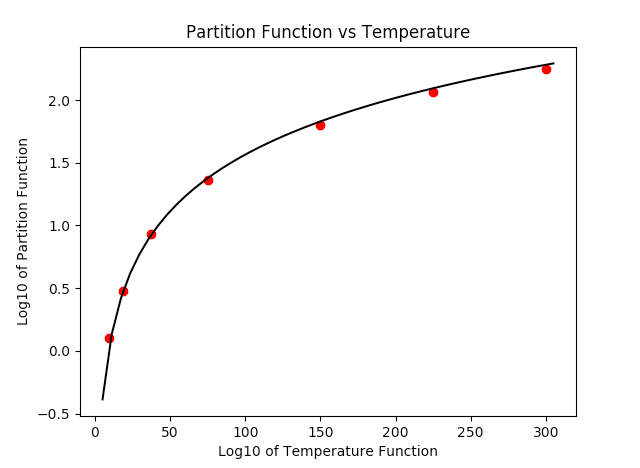
The resulting plot from the example above
Querying the Catalog with Regexes and Relative names
Although you could print the species table and see what molecules you’re
interested in, maybe you just want a general search of any H2O molecule,
or maybe you want a specific range of H2O molecules in your result. This
module allows you to enter a regular expression or string as a parameter
by adding the parameter parse_name_locally = True and returns the results
that the regex matched with by parsing through the local catalog file. It is
recommended that if you are using just the corresponding molecule number found
in the JPL query catalog or a string with the exact name found in the catalog,
that you do not set the local parse parameter since the module will be able
to query these directly.
>>> from astroquery.jplspec import JPLSpec
>>> import astropy.units as u
>>> result = JPLSpec.query_lines(min_frequency=100 * u.GHz,
...                              max_frequency=1000 * u.GHz,
...                              min_strength=-500,
...                              molecule="H2O",
...                              parse_name_locally=True)
>>> print(result)
    FREQ      ERR     LGINT    DR    ELO    GUP  TAG   QNFMT   QN'      QN"
    MHz       MHz    nm2 MHz        1 / cm
----------- -------- -------- --- --------- --- ------ ----- -------- --------
115542.5692   0.6588 -13.2595   3 4606.1683  35  18003  1404 17 810 0 18 513 0
 139614.293     0.15  -9.3636   3 3080.1788  87 -18003  1404 14 6 9 0 15 312 0
 177317.068     0.15 -10.3413   3 3437.2774  31 -18003  1404 15 610 0 16 313 0
 183310.087    0.001  -3.6463   3  136.1639   7 -18003  1404  3 1 3 0  2 2 0 0
...
Length = 2000 rows
Searches like these can lead to very broad queries, and may be limited in response length:
>>> print(result.meta['comments'])
['', '', '', '', '', 'form is currently limilted to 2000 lines. Please limit your search.']
Inspecting the returned molecules shows that the ‘H2O’ string was processed as a regular expression, and the search matched any molecule that contained the combination of characters ‘H2O’:
>>> tags = set(abs(result['TAG']))  # discard negative signs
>>> species = {species: tag
...            for (species, tag) in JPLSpec.lookup_ids.items()
...            if tag in tags}
>>> print(species)
{'H2O': 18003, 'H2O v2,2v2,v': 18005, 'H2O-17': 19003, 'H2O-18': 20003, 'H2O2': 34004}
A few examples that show the power of the regex option are the following:
>>> result = JPLSpec.query_lines(min_frequency=100 * u.GHz,
...                              max_frequency=1000 * u.GHz,
...                              min_strength=-500,
...                              molecule="H2O$",
...                              parse_name_locally=True)
>>> tags = set(abs(result['TAG']))  # discard negative signs
>>> species = {species: tag
...            for (species, tag) in JPLSpec.lookup_ids.items()
...            if tag in tags}
>>> print(species)
{'H2O': 18003}
As seen above, the regular expression “H2O$” yields only an exact match because the special character $ matches the end of the line. This functionality allows you to be as specific or vague as you want to allow the results to be:
>>> result = JPLSpec.query_lines(min_frequency=100 * u.GHz,
...                              max_frequency=1000 * u.GHz,
...                              min_strength=-500,
...                              molecule="^H.O$",
...                              parse_name_locally=True)
>>> tags = set(abs(result['TAG']))  # discard negative signs
>>> species = {species: tag
...            for (species, tag) in JPLSpec.lookup_ids.items()
...            if tag in tags}
>>> print(species)
{'H2O': 18003, 'HDO': 19002, 'HCO': 29004, 'HNO': 31005}
This pattern matches any word that starts with an H, ends with an O, and contains any character in between.
Another example of the functionality of this option is the option to obtain results from a molecule and its isotopes, in this case H2O and HDO:
>>> result = JPLSpec.query_lines(min_frequency=100 * u.GHz,
...                              max_frequency=1000 * u.GHz,
...                              min_strength=-500,
...                              molecule=r"^H[2D]O(-\d\d|)$",
...                              parse_name_locally=True)
>>> tags = set(abs(result['TAG']))  # discard negative signs
>>> species = {species: tag
...            for (species, tag) in JPLSpec.lookup_ids.items()
...            if tag in tags}
>>> print(species)
{'H2O': 18003, 'HDO': 19002, 'H2O-17': 19003, 'H2O-18': 20003, 'HDO-18': 21001}
This pattern matches any H2O and HDO isotopes.
Troubleshooting
If you are repeatedly getting failed queries, or bad/out-of-date results, try clearing your cache:
>>> from astroquery.jplspec import JPLSpec
>>> JPLSpec.clear_cache()
If this function is unavailable, upgrade your version of astroquery.
The clear_cache function was introduced in version 0.4.7.dev8479.
Reference/API
astroquery.jplspec Package
JPL Spectral Catalog
- author:
Giannina Guzman (gguzman2@villanova.edu)
- author:
Miguel de Val-Borro (miguel.deval@gmail.com)
Classes
|
Configuration parameters for |